Configuring inference process

There are two ways of interacting with HeaRTDroid:

Using Java API
Using HaQuNa commandiline shell

Both of these methods are equivalent, although Java API allows for more flexibility than commandline shell, obviously. Below thee two approaches are described with the emphasis on three most important factors that impacts the reasoning:

Switching reasoning modes.
Switching method for evaluation of logical formulae.
Switching conflict set resolution strategies.

Use case

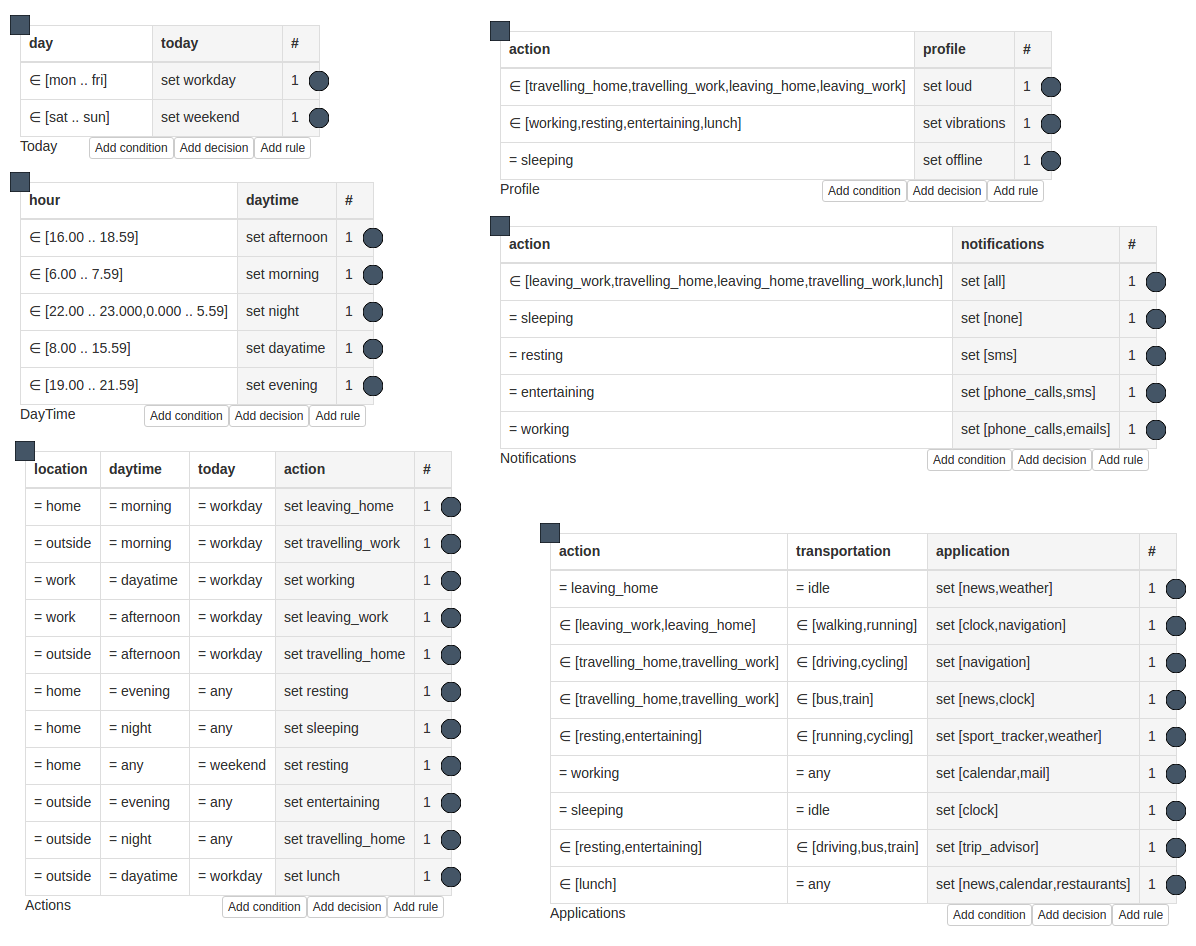
For the purpose of this tutorial we will use the simplified (and not completed) version of a model presented in: Uncertainty handling in rule-based mobile context-aware systems. The model uses informatio about current time, day and user location and transportation mode to derive either the applications that should be recommended to the user, mobile phone profile (silent, loud, vibrations, etc.), or types of notifications that should be presented to the user on the locked screen. These three different decisions are produced by three separate tables: Application, Profile and Notification, respectively. The full model is presented in the Figure below:

The HMR file with callbacks for obtaining hour and day of a week can be downloaded from here.

HeaRTDroid supports three different types of inference: Fixed order, Data driven and Goal driven. We should chose the inference mode depending on the goal we want to achieve. The next section discusses different use case scenarios to demonstrate when each of the reasoning modes is useful.

Reasoning options

Reasoning modes

There are three reasoning modes available in HeaRTDroid:

Fixed-Order (FOI), which is the simplest algorithm that consists of a hard-coded order of XTT2 tables to process. In this mode, the system has to pass to HeaRTDroid explicit, ordered list of tables to be processed.
Data-Driven (DDI), which can be used to find all possible information that can be inferred from given data. This mode is similar to forward chaining inference. In this mode, the system needs to pass to HeaRTDroid only the starting tables, and the engine will crawl the XTT2 network to search for tables that are successors of the initial tables, until no further tables could be found.
Goal-Driven (GDI), which can be used to find only a specific information that can be inferred from a specific subset of XTT2 tables. This mode is similar to backward chaining inference. This mode is kind of opposite to DDI mode. The system needs to pass to HeaRTDroid the table(s) that produce(s) desired conclusions, and the engine crawls backward to find all the tables that are needed to derive the conclusion.

In the following Figure DDI and GDI inference modes were presented (FOI was skipped, being trivial). In the Figure, every mode can be tokenized, meaning that only tables with sufficient number of tokens can be processed. This feature is not yet released in stable version.

The following paragraphs gives more intuition on when each of these modes is useful.

When to use FOI mode?

In FOI mode, the list of tables to process is given explicitly. No additional crawling over the network of tables is done, hence this mode is the fastest one. In case when each reasoning cycle has to process specific set of tables is specific order that do not change – this mode might be a best choice.

It can also be useful for testing the model, since you can separately run the inference on different tables to see how they handle incomplete or uncertain data.

This mode may also be useful if you use looped tables (i.e. tables that uses the same attribute in conditional and in decision part. Such tables are not recommended, but possible) along with the uncertainty management for cumulative rules (i.e. rules that use the same attributes in decision part, but are spread over different tables – see Managing uncertainty with Certainty Factors Algebra tutorial) This is because in the DDI and GDI modes the order of tables that have the same schemas is non-deterministic. However, the order may be important in case of looped tables and uncertainty evaluation.

When to use DDI mode?

In DDI mode the engine treats the XTT2 network as a directed graph and uses BFS algorithm to build the list of tables to process. It takes as a parameter a subset of these tables from which the inference should start. The BFS algorithm is then launched treating every initial table as a starting node. Every table that the algorithm visits is placed on a list $V$ in such a way that the paths generated by subsequent BFS launches are concatenated to the beginning of the list. This assures that the order of the tables will be correct according to forward-chaining paradigm.

The DDI inference strategy interprets the XTT2 model as a direct graph, in which the edges between tables are determined by their schemas. The edges are directed according to the following pattern. If schema of a table $v$ is defined as $(\mathbb{COND}, \mathbb{DEC})$ , then the edge from this table to all tables with schema $(\mathbb{COND}_n, \mathbb{DEC}_n)$ , such that $\mathbb{DEC} \cap \mathbb{COND}_n \neq \emptyset$ is created. Finally, all the elements from list $V$ are placed on the stack. The stack is then rewritten into resulting stack $S$ in reverse order.

This mode is useful, if the model can change over the time, but the initial tables would not. In such a case the explicit list of tables is not possible to be given a priori, bu the DDI mode can build it dynamically. Also, it may be useful when the number of tables to process is relatively large and listing them explicitly might be difficult.

When to use GDI mode?

The GDI mode is similar to DDI mode. The user (or system) gives the algorithm a list of tables (or single table) that produce desired conclusions. Every table that the algorithm visits is placed on a list $V$ in such a way that the paths generated by subsequent BFS launches are concatenated to the beginning of the list However, it differs in a way the direction of graph edges is interpreted. The edges are directed according to the following pattern. If schema of a table $v$ is defined as $(\mathbb{COND}, \mathbb{DEC})$ , then the edge from this table to all tables with schema $(\mathbb{COND}_n, \mathbb{DEC}_n)$ , such that $\mathbb{DEC}_n \cap \mathbb{COND} \neq \emptyset$ is created. Finally, all the elements from list $V$ are placed on resulting the stack $S$ .

This mode is useful, if the model can change over the time, but the initial tables would not. Additionally, this mode may com in handy when you have a model that produces a lot of different conclusions, but not all of the conclusions are needed in each reasoning cycle.

As an example take the model presented at the beginning of this tutorial. There are three tables that produce different conclusions: Application, Notification and Profile. However, sometimes the system may only need the application recommendation. In such a case processing of Notification and Profile tables will be waste of resources, but also will end up in firing rules which are not related to the actual goal of the invoked inference.

This is when the GDI inference should be used. By specifying which table is the goal table, the system will automatically collect all other tables that are needed to perform reasoning, i.e. Today, DayTime and Action.

Uncertainty evaluation

There are three types of evaluation of rules in HeaRTDroid:

Deterministic, that is based on ALSV(FD) logic. This is regular logic-based reasoning, where each formulae can be either true or false.
Uncertain, with certainty factors algebra. This method was more broadly described in Managing uncertainty with Certainty Factors Algebra tutorial.
Uncertain, with probabilistic interpretation of XTT2 tables. This mode is not part of the engine itself, but is supported by the external module. Read more on this mode in Managing uncertainty with Bayesian networks tutorial.

Both interaction methods (HaQuNa and Java API) support two first modes. The third mode is available as a separate module and can be used either as a standalone application, or as a library via Java API.

Conflict set resolution

Conflict set is understood as a set of rules that have their conditions fulfilled. Different behaviors of the inference engine could be desired in such situations. In HeaRTDroid there are three basic types of conflict set resolution mechanisms, that can work differently depending which uncertainty handling mechanism was chosen. These conflict set resolution strategies are:

First – Only the first rule from the XTT2 table that has its conditions fulfilled is fired.
Last – Only the last rule from the XTT2 table that has its conditions fulfilled is fired.
All – All the rules with fulfilled conditions are fired.

The behavior of these strategies changes (or is modified) if uncertainty handling with CF algebra is turned on. In CF evaluation, the rules from the single table are divided into subsets, such that rules that produce the same conclusion (i.e. sets exactly the same value to the attribute from conditional part) are in the same subset. The conflict resolution is applied to these subsets, not to the XTT2 table as a whole. In such a case it may happen (it probably will) that several rules from a single table will be fired even when selecting First or Last strategies.

Reasoning with HaQuNa

Please refer to HaQuNa tutorial.

Reasoning with Java API

Please refer to HeaRTDroid quickstart section.

HeaRTDroid

Sidebar

Table of Contents

Configuring inference process

Use case